Introduction

This is a quick tutorial for visualizing and developing a basic understanding of simple random walks, branching processes, and regime switching. As this is geared toward individuals who may not have taken a probability course yet, we’re not going to get deep into the math here (Although if you are interested in the maths, Gordan Zitkovic’s Stochastic Processes notes can explain all of that better than I ever could). Rather, we’re going to simulate these processes to see what is actually occurring over time.

Before we start, you might ask why we even care about random processes. Given that “because random processes are NEATO” isn’t a satisfying answer for most people, let’s consider some practical applications. We can use random walks to approximate price fluctuation in the stock market or to simulate the movement of molecules in liquids and gasses. Branching processes are useful for modeling reproduction, and the probability that a certain population will go extinct. I personally have made use of random processes as part of my ongoing attempts to automatically map the Antarctic Ice Sheet.

In this tutorial we aren’t going to apply these concepts to any problems – that will come later. Rather, we’re just going to visualize them in order to build up our intuition about what is happening behind all the maths.

Simple Random Walks

A simple random walk with parameter is a sequence of random variables with the following properties:

1. 
2. is independent of
3. The random variable has the following distribution:

Basically, at each time n+1, we take a step up with probability p or a step down with probability (1 - p).

We can visualize this process in R using just a few lines of code.

# set probability of moving up at time t+1
# initialize set of moves and position at time = 0
p = 0.5
s = 0
s[1] = 0


# generate N = 100 random values from a Uniform(0,1) distribution
# assign 1 if < p, -1 if >=p
N = 100

for(i in 2:N)
{
x = runif(1)
if(x<p) {s[i]=s[i-1]+1} else {s[i]=s[i-1]-1}
}  

# generate basic plot
plot(s, type ="l")

What does this actually look like, though? Let’s look at plots for p = 0.4, 0.5, and 0.9.

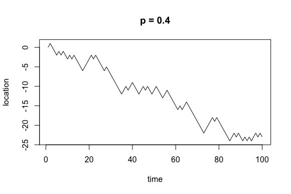
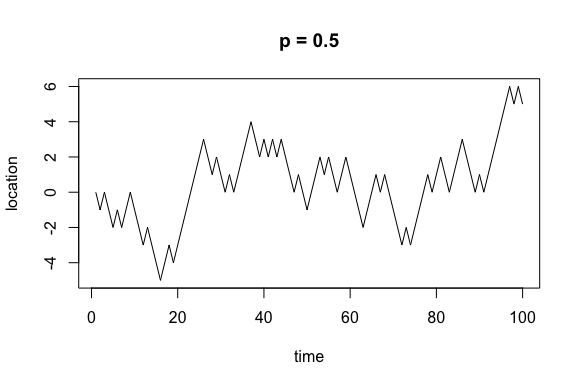
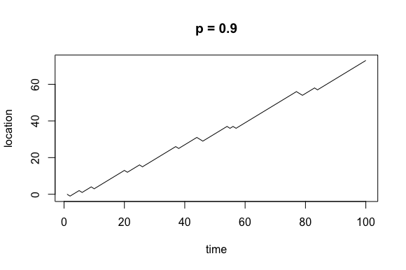
Now, it’s important to remember that while these processes are beholden to some probability distribution, they are random. For any random walk with parameter p I could run the simulation 10 times and produce 10 different plots.

Branching Processes

Every once in a while a mathematical concept will arise from an individual with problematic views, and the branching process is one of them. Sir Francis Galton, also known as the father of eugenics, questioned how many male children each generation of a family would have to produce on average in order for the family line to not become extinct. After a collaboration with Henry William Watson, the branching process model was born.

Thankfully, branching processes have applications outside of eugenics. For example, we can use them to model whether a population of cancerous cells will become extinct before it grows large enough to overwhelm the surrounding tissue.

Modeling a Single Branching Process

To model a branching process we want to start with a single individual, , at time n = 0, and assume that they will produce a random number of children before dying off. The number of children they can produce may only be a nonnegative integer, so we will model this random variable using a Poisson distribution with parameter lambda, where lambda is the expected value.

If our initial individual produces 0 children, the population is dead and nothing will happen at any time going forward. If they produce > 0 children, the children will then go on to reproduce as well. If none of them produce children, the population dies off. Otherwise, at time n = 2 we will have individuals in the population. If it ever happens that Z_n = 0, our population is extinct. Otherwise, .

When I first learned about branching processes I found it difficult to really visualize what’s going on simply based on the math, and coding it up really helped me out. So let’s look at the code and generate some plots!

#over multiple trials we will show that if population does not immediately die off it will explode

#initialize list of population size at generation n
Z<-1

#pop. size 1 at generation 0
Z[0] = 1

#poisson r.v.
#each member generates poisson(lambda) offspring
#sum offspring
lambda = 2
N = 20

Z[1] = rpois(Z[0], lambda)

for (i in 2:N)
{
  if(Z[i-1]==0) {Z[i]=0} else
    {
      x=rpois(Z[i-1], lambda)
      Z[i] = sum(x)
    }
}
Z
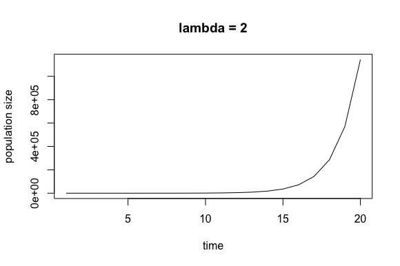
plot(Z, type = "l")

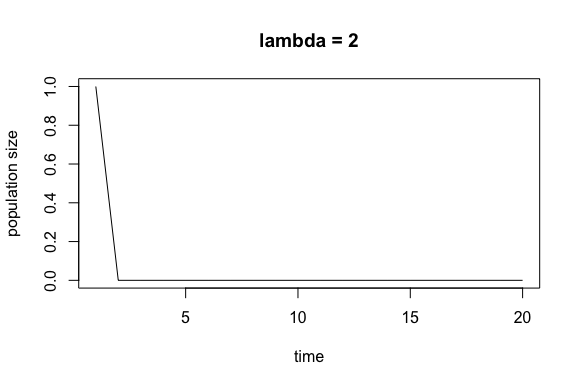
I like to run this simulation using lambda = 2 because over multiple trials we can clearly see that if the population does not die off within the first few generations, it will explode. See the plots below.

Approximating the Probability of Extinction

Since branching processes are random, running a single simulation is rather worthless if we’re seeking some kind of concrete information. For example, one question we could ask is what is the probability that population reproducing itself from a Poisson(2) distribution will become extinct?

If you’ve taken a class on stochastic processes then you know we can find this probability using generating functions, but what if you don’t know what a generating function is?

Well, if we can simulate one branching process, we can simulate hundreds of branching processes and thus approximate the probability of extinction.

After simulating a Poisson(2) branching process 300 times, I found that the extinction probability is around 0.2, which is the same solution we would find using the generating function .

Regime Switching

What if we want to consider a system that has only two states? Some examples of such a system would be high/low volatility in a financial market, english/non-english text in a work of literature, or my personal favorite example, the presence of water or no water underneath an ice sheet.

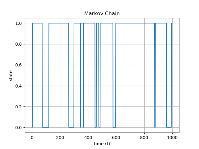
We can represent these states as 0 and 1 and then construct a stochastic matrix where and are the probabilities of remaining in the current state and and are the probabilities of switching states:

The plot below was generated using the stochastic matrix

Ref

• My own personal notes from Stephen Walker’s Stochastic Processes class at UT Austin
• Gordan Zitkovic’s lecture notes on random walks and branching processes