Hey y’all! Today I’m going to talk about some of the first steps I took when I was trying to figure out how to tackle my ice radar project. I wrote up an introduction to that project in The Ice Radar Chronicles Part 1, but to give a quick summary, I have a bunch of radar images of the Antarctic Ice Sheet, and I want to speed up (and eventually fully automate!) the process of using those images to determine where the upper and lower boundaries of the ice are located.
The raw radar files are pretty massive so while I was exploring the data and testing out some theories, I just left it in screenshot form. I have some more sophisticated plans, but I’ll save those for a future post. :)
Edge Detection
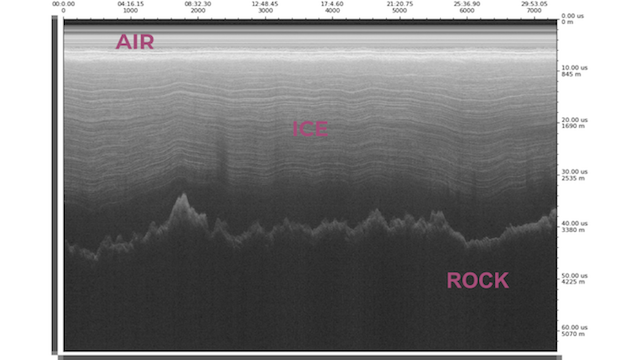
My first thought was that edge detection might be useful. I had two two different possible end goals in mind: the first, more obvious goal, was to just segment the radar transect into air/ice/rock (or water, in the case of floating ice). I also thought it would be neat to output an interactive contour map which would not only capture the air-ice interface (surface) and ice-rock interface (bed), but also the layers that sometimes show up in the ice. A lab tech could then select the contours that represent their feature of interest.
My main concern regarding edge detection was that radar images can get weird. Sometimes they’re basically visually perfect, like the one above. But ice has its quirks, and so often radar images will contain artifacts caused by the radar reflecting off water, salt, crevasses, buildings (I’m looking at you, South Pole Station), and volcanic ash plumes. Sometimes the radar signal is just straight up weak or nonexistent, due to depth, temperature, or the slope of the bottom of the ice. But scikit-image has a super convenient built in canny edge detection fuction, so I figured it wouldn’t hurt to give edge detection a try on one of the more visually perfect transects.
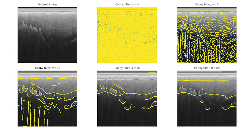
There are several steps to Canny edge detection. First, we want to filter out excess noise that might result in false edge detection. The Canny filter does this by applying a Gaussian filter with some user-defined standard deviation to smooth the image. It then finds the intensity gradients of the image and “thins” potential edges using non-maximum suppression, which suppresses gradient values other than the local maxima. Finally, pixels with a gradient value below some user-defined lower threshold are suppressed, leaving “strong” edge pixels (those with a gradient value above some user-defined upper threshold) and “weak” edge pixels (those with a gradient value between the two thresholds). The filter extracts all of the strong edge pixels and some of the weak edge pixels and finally outputs a 2-D binary array edge map. See below for canny edge maps using varying Gaussian filters applied over the original radar image.
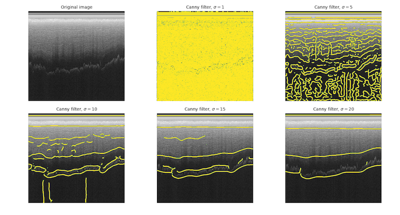
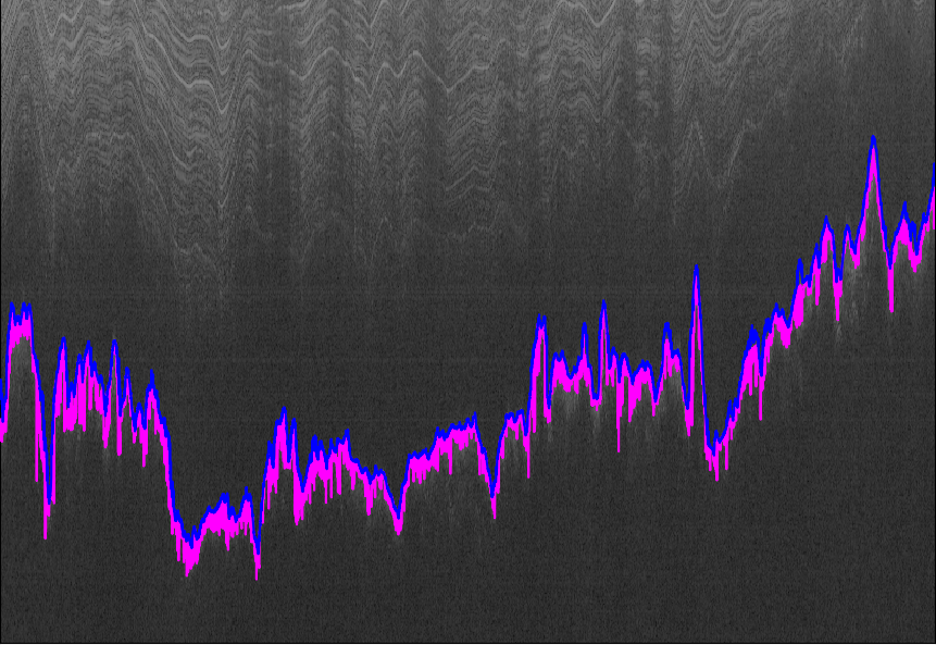
The canny filter with standard deviation 10 actually did a pretty good job of capturing the upper and lower boundaries of the bed. I used our regular picking software to approximate what those boundaries would look like if they were cleaned up a little bit to be continuous, and then I compared that output to the output generated from my own picks. It was more noisy than I prefer, but otherwise surprisingly decent. In the image below, the bed as found by my picks is in blue, and the the bed found by the cleaned up edge detection picks is in pink.
So, I said that these results were surprisingly decent, but recall that I tested edge detection on an ideal image. When I ran it on a less visually perfect (but still REALLY nice, as far as radar images go) transect, my results were pretty useless.
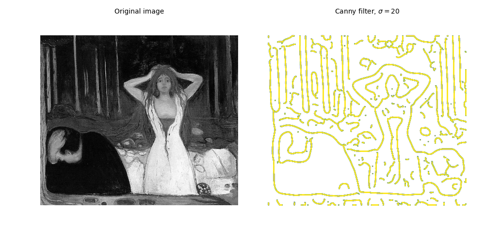
There are several other edge detection methods, but at this point I think it’s a good idea to move on and try something new. I’ll have another post up soon, but until then here’s a canny filter applied to one of my favorite Edvard Munch paintings. :)